Guidelines
Measuring computational cost
The cost of the computation should be expressed in work units. TauBench should be run at least three times in sequential mode to obtain an average wall clock time T1. Then track the wall clock time taken by your CFD solver (excluding the initialization, post-processing data preparation time and file I/O time) T2. The work unit is then defined as NP*T2/T1, where NP is the number of processors involved in the computation. When running TauBench, use the following parameters:
>> mpirun -np 1 ./TauBench -n 250000 -s 10
Resolution
The length scale h in all computations will be defined as (N)1/d, with d the dimension of the problem and N the total number of degrees of freedom, unless specified otherwise.
Running computations
-
For steady problems, start your computation from a uniform free-stream unless otherwise specified. Use the L2 norm of the global residual to monitor convergence. Steady state is assumed if the initial residual is dropped by 10 orders of magnitude. For cases impossible to converge 10 orders, 8 orders can be used as a convergence criterion.
-
Far-field boundaries should not implement a vortex correction.
Computational meshes
The gmsh format (http://www.geuz.org/gmsh/doc/texinfo/gmsh.html) is adopted for the workshop. A mandatory set of meshes will be provided for the baseline cases, which can be complemented with unstructured meshes at similar resolutions. These are usually also provided by the test case leader, but can be generated by the participants as well. For advanced cases, test case leaders will provide suitable meshes on request. If you generate new meshes, please respect the domain definition used/specified by the test case leaders (eg. for the provided meshes).
Error computation
For any solution variable (preferably non-dimensional) s, the L2 error is defined as (Option 1)
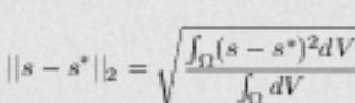
For an element or cell based method (FV, DG etc), where a solution distribution is available on the element, the element integral should be computed with a quadrature formula of sufficient precision, such that the error is nearly independent (with 3 significant digits) of the quadrature rule. Note that for a FV method, the reconstructed solution should be the same as that used in the actual residual evaluation.
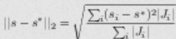
For a finite difference scheme, the error is defined using the Jacobian matrix J
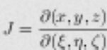
as (Option 2)
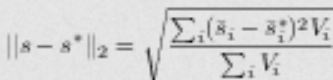
For some numerical methods, an error defined based on the cell-averaged solution may reveal super-convergence properties. In such cases, we suggest another definition (Option 3)
Contact:
info cenaero [dot] be (info[at]cenaero[dot]be)